

Hi!
This is the Science Scribbler Team with a new update to our latest project: Key2Cat. As you might have seen from our last blogpost, we have arrived at the second stage of our workflow, which is called ‘classification’. It helps us to refine the data we have gathered from the particle picking workflow and allows us to prepare it for our deep learning algorithm. Many of you have tackled the new workflow in which you were asked to classify instances shown in the centre of the green circle:

Every single mark from the particle picking workflow generated an individual image area as shown on the left hand side above, and each image area was reviewed by five volunteers. Given that we have thousands of nanoparticles and clusters within our Au/Ge dataset, one quickly realises that the number of required classifications is tremendous – 362,693 to be precise.
Nonetheless, you dashed through the Au/Ge dataset like a storm! Once more we would like to
-Thank you for this enormous effort!-
CONNECTING THE DOTS
For the Au/Ge system specifically, we have basically collected all of the required data to build a new training dataset for our deep learning algorithm. As per usual in science, there are a number of things that can be expected from the data, whilst there are some features which are more surprising. We have started to explore algorithms to group marks into centroids of nanoparticles and clusters and tested first approaches to assign the classes given by all volunteers.
Let us compare an original raw image and all marks given by our volunteers:

We promise, that this is a particularly great example J. Each of the tiny green circles in Figure 1b represents a single mark given by a volunteer on a smaller image area that was presented in the first workflow. The number of circles is particularly high at the centres of individual nanoparticles or nanoparticles that make up a cluster – a great sign!
By going through the data stack, we have written some processing code to connect the individual marks (Figure 1b) to classes given in the second workflow. These were given as:
| Class | Numerical value |
| Nanoparticle | 0 |
| Cluster | 1 |
| Artifact | 2 |
| Nothing/Something else | 3 |
Currently, we have grouped together the classes of ‘Nothing’ and ‘Something else’ into a unified class as we wanted to focus on particle instances at first. Once the marks are connected to the classes, we can visualise them by assigning different colours. Here is our exemplary image in full resolution:
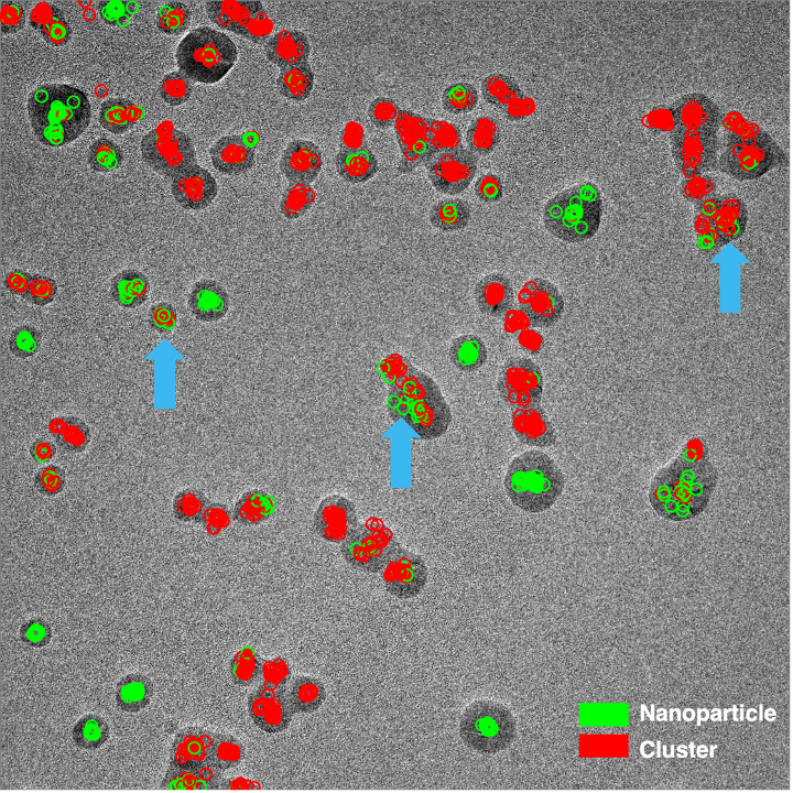
What an impressive result! We can clearly see that you have been able to distinguish nanoparticles and clusters really well. Despite the complexity of the image, i.e. having multiple cases of both nanoparticles and clusters in the vicinity of each other, classes were assigned correctly in the large majority of cases.
However, it is quite difficult to distinguish the centroids of the individual nanoparticle instances. Moreover, there are a few cases where volunteers were of mixed opinion (consider blue arrows given in Figure 2). How do we arrive at one centroid per instance with a definitive, single label?
PINNING DOWN THE CLUSTERS
There are different approaches and algorithms that can be applied. Starting from earlier trials that included the K-Means algorithm, we have tested different approaches. At the moment, the most promising one is the HDBSCAN algorithm. Briefly, it extends the popular DBSCAN algorithm into a hierarchical clustering algorithm. A more detailed explanation is given by the authors on their package webpage.
Naturally, there are a lot of parameters one can play with and all of them have an influence on the output obtained. We are still in the phase of grid-searching for the optimum solution, but the ones we have set empirically have already given remarkable results. In particular, we have set the minimum points required to form a centroid to 11, because due to how we tiled our data, each particle instance was seen four times by five volunteers. Hence there should be a total of 20 picks per nanoparticle instance arising from different tiles of our data, with 11 raising a majority. This is actually visible in some of the nanoparticles in Figure 2 as well: Whilst in some cases all marks were put on nearly the exact same spot, other cases appear more decentralised.
Running the HDBSCAN algorithm and assigning a single class to a given centroid by majority principle, we arrive at the following result:
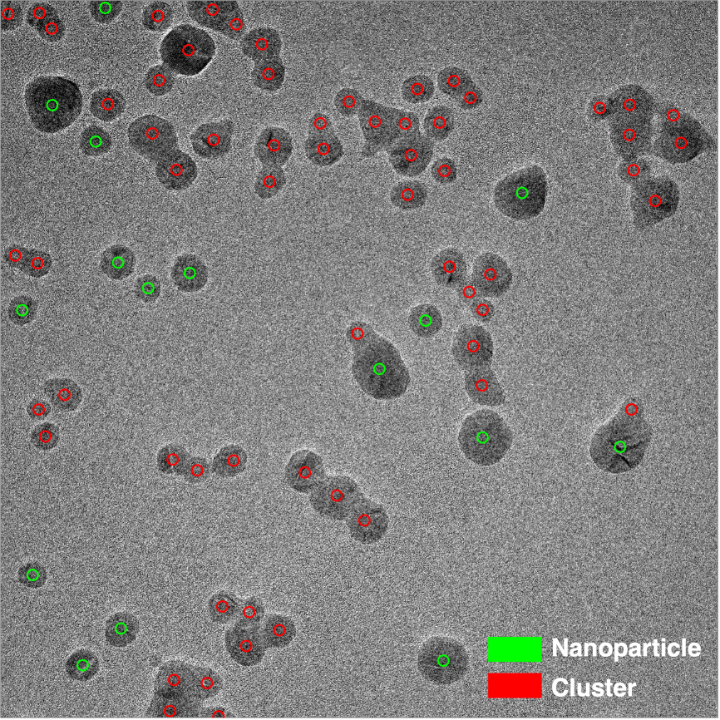
Apart from very few exceptions, we already arrive at a very promising result at this stage! Without your help this would have not been possible – once again we would like to thank you for all your time and effort so far!
WHAT IS NEXT?
Now we have to look more closely at optimising the results. Tricky cases could include examples like these:

Naturally, the obtained mixed result is dependent on how we processed our data. However, in order for this result to be consistent throughout our grid-search, how do we find a rule to decide on a class for similar instances? As it stands, for these examples, it’s a 50:50 split between ‘nanoparticle’ and ‘cluster’.
While we get to work on optimisation, we are eagerly awaiting the results of our current active workflow, the Pd/C classification. We invite you to pop-by and leave a few classifications! J
Follow this link to classify. You can also get in touch with us on the Key2Cat Talk forums.
That’s it for now – we are looking forward to updating you again soon!
-Kevin & Michele
